 |
MRS
1.0
A C++ Class Library for Statistical Set Processing
|


|
|
MRS
1.0
A C++ Class Library for Statistical Set Processing
|
|
An adaptive histogram is a histogram where bin widths and bin centres of the partition of the data space adapt in some way to the data to be represented in the histogram. The basic ideas here are from classical statistical principles.
The AdaptiveHistogram class organises statistical sample data for the purpose of creating adaptive histograms. The class holds the container of sample data and uses a tree of SPSnodes (StatsSubPaving) to represent a regular non-minimal subpaving or partition of the dataspace which can develop adaptively according to the data.
The AdaptiveHistogram object manages the tree through the tree's root node. This represents the box being covered by the subpaving, which is the data sample space to be partitioned into histogram bins. The boxes of the statistical subpaving can be considered as histogram bins and are represented by the leaf nodes of the tree. Data is associated with boxes in the subpaving: the count of data associated with a leaf node of the tree is the number of data points falling into the box (bin) represented by that node.
The AdaptiveHistogram data member holdAllStats controls whether the tree of SPSnodes managed by the histogram object will maintain all summary statistics for the data in each node, or just count data. If a value for holdAllStats is not specified in the AdaptiveHistogram constructor, holdAllStats will be set to false so that, by default, only count data is maintained.
The image belows shows a partition of a [0, 1]x[0, 1] data space into a subpaving and the data points in each box of the subpaving, together with the tree representation with the counts of data in the boxes represented by each node of the tree. In the image, the nodes of the tree are identified with their nodeNames.
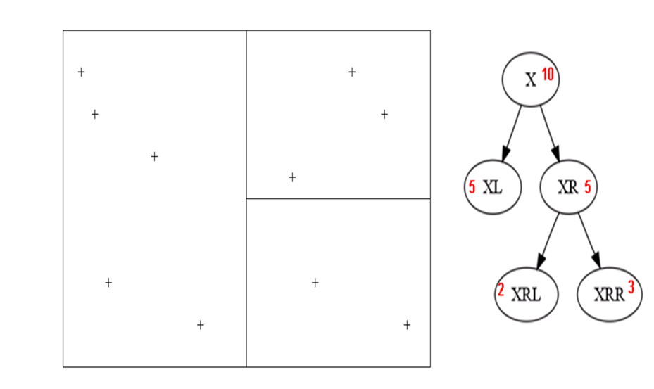
The equivalent normalised histogram is shown below. The height  associated with bin
  is
is  where
where  is the number of data points associated with bin j,
  is the volume of bin j, and
  is the total number of data points in the histogram,
  . Thus
![\[ sum_{bins j} h_jvol_j = 1 \]](form_15.png)
The AdaptiveHistogram class declarations and definitions can be found in adaptivehistogram.hpp and adaptivehistogram.cpp.
The purpose of the AdaptiveHistogram class is to allow the histogram bin widths and bin centres to adapt in some way to the data to be represented in the histogram.
There are three ways in which a partition can be formed:
We can use a priority queue to form the partition starting from the point where all the data is initially associated with a single root box (the sample data space). The subpaving is refined by progressively bisecting boxes using a priority queue to determine which box, of all the boxes in the subpaving at that point, to bisect next. Using the tree representation the priority queue operates on leaf nodes, prioritising leaf nodes for splitting.
The priority queue operation must be able compare SPSnodes in order to prioritise which to act on first. Priority queue methods of the AdaptiveHistogram class use a function object for comparing SPSnodes. NodeCompObj is an abstract base class from which concrete classes for these function objects must be derived. Some examples of useful node comparison function objects can be found in the file nodecompobj.hpp.
The priority queue operation must also have a 'stopping rule' to stop further changes in the subpaving/its tree representation. Typically this rule uses characteristics of the histogram as a whole (for example, the number of leaves in the tree). Priority queue methods of the AdaptiveHistogram class use a function object to provide the stopping rule. HistEvalObj is an abstract base class from which concrete classes for these function objects must be derived. Some examples of useful function objects to determine when adaptive changes in the data partition should cease can be found in the file histevalobj.hpp.
The operation of the priority queue can be further controlled by specifiying a minimum number of data points which can be associated with any node in the tree which will be created by the method. Setting this parameter to be a value > 0 will effectively remove from the queue any node which cannot be split because that would result in a child leaf with less than the required minimum number of data points associated with it. The priority queue operation will cease when there are no nodes in the queue if this occurs before the stopping rule is satisfied. Thus 'large' nodes (on the basis of the node comparison function) may not be split and the tree may not yet satisfy the stopping rule when the priority queue method has finished because of the effect of the value supplied for the minimum number of data points to be associated with a node.
The prioritySplit method also takes a parameter minVolB which controls the minimum volume of the boxes represented by the nodes in the tree which will be create by the method. If the total number of data points associated with the whole tree is N, then the minimum volume of the box represented by any node will be  . Setting minVolB to 0.0 will mean that there is no minimm volume restriction on the boxes. The minimum volume parameter is useful when priority queue splitting to optimise some histogram fit scoring formula such as Akaike's Information Criteria (AIC).
Some care must be taken to specify a compatible pairing of node comparision and stopping rule, to ensure that the number of nodes in the queue will not just continue to increase without the stopping rule being satisfied.
For splitting using a priority queue method documentation see AdaptiveHistogram::prioritySplit.
Priority queues can also be used to coarsen a partition by reabsorbing pairs of sibling leaf nodes back into their parent node. This is known as 'merging' a subpaving. For merging using a priority queue method documentation see AdaptiveHistogram::priorityMerge.
For examples using priority queue approaches see An AdaptiveHistogram with Bivariate Gaussian data and Example using data from a RSSample object
The histogram partition can be progressively refined as each data point is inserted if the rules for forming the partition can be applied directly to each node in the tree representing the subpaving. For example, a statistically equivalent blocks (SEB) partition which has a maximum of some specified number of data points associated with each bin can be formed in this way. Each leaf node representing a box in the subpaving will be split when the number of data points associated with that node exceeds the maximum, irrespective of the attributes of other nodes or of tree as a whole.
Since each SPSnode in the tree can behave autonomously in this situation, the decision on whether to split is 'delegated' to the SPSnode objects. The SPSnode class provides a method for associating data with a node which takes as a parameter a function object which will direct whether the node should split after the data is added. SplitDecisionObj is an abstract base class from which concrete classes for these function objects must be derived. Specific splitting rules can be encoded using these function objects and then used by the method for inserting data into an SPSnode. The total regular subpaving/its tree representation will develop accordingly. Some examples of useful function objects that can be used by nodes to determine when to split can be found in the file splitdecisionobj.hpp.
See An AdaptiveHistogram with Bivariate Gaussian data for an example using this kind of process for partition formation.
The AdaptiveHistogram class can probabilistically change its partition to form different histogram states in a MCMC process. For more details see AdaptiveHistogram::MCMC and AdaptiveHistogram::MCMCsamples documentation.
The AdaptiveHistogram class is designed to deal with multi-dimensional data. Data associated with each AdaptiveHistogram object is stored as the cxsc::rvector type.
The AdaptiveHistogram class provides methods to take data from appropriately formatted txt files, from a collection of doubles, from a container of rvectors, or from an RSSample object. If necessary, direct data insertion can also be coded in the user program. Some of these methods are discussed in more detail below. Refer to the AdaptiveHistogram class documentation for more detail.
When data is input to a AdaptiveHistogram object an attempt will be made to associate it to the StatsSubPaving managed by the histogram. If the data does not fit in the root box of this StatsSubPaving, it cannot go into the StatsSubPaving. Any data successfully associated with the StatsSubPaving managed by the histogram will be put into the AdaptiveHistogram object's data collection.
If the AdaptiveHistogram does not have a StatsSubPaving to manage when the data is inserted, one will be created with a root box of the appropriate size and dimensions to fit all the input data matching the dimensions expected by the input method used.
This method reads in lines of data representing rvectors from a txt file. The dimensions of the rvector are either specified by the user or deduced from the input data format. All the data is then expected to be in the same dimensions. Any data line read which is less than the expected dimensions will be rejected (if a data line with more values than the expected dimensions is read, the excess values will be silently ignored).
See An AdaptiveHistogram with Bivariate Gaussian data for an example creating a txt file of data and then using this input method.
The method expects one line per rvector with the elements separated by white space (space or tabs) or commas (","), with no non-numeric characters ('e' and 'E' are accepted as part of a floating point format).
The method can read one-dimensional and multidimensional data.
The method carries out some basic data checking. Input lines which do not pass (because they contain illegal characters, or where the data is not of the expected dimension) are printed to standard error output with an error message but the entire file will continue to be processed until the end of the file is reached.
For example
For method documentation see AdaptiveHistogram::insertRvectorsFromTxtOrd. Note that different levels of checking are available with insertRvectorsFromTxtParanoid and insertRvectorsFromTxtFast.
Data can be input directly from a collection of containers of type VecDbl.
As with data input from txt files, the dimensions of the rvector are specified by the user or deduced from the input data and all the data is then expected to be in the same dimensions. Any VecDbl containing less than the expected dimensions will be rejected (if a VecDbl with more values than the expected dimensions is found, the excess values will be silently ignored).
For method documentation see AdaptiveHistogram::insertRvectorsFromVectorOfVecDbls.
This method may be useful when reading in output from other programs which do not use the cxsc::rvector type.
Data as rvectors can be input directly from a container of type RVecData. For method documentation see AdaptiveHistogram::insertFromRVec.
For an example using this data input method see Example of averaging histograms
A sub-sample of the data in a container of type RVecData can also be input to the histogram. See AdaptiveHistogram::insertSampleFromRVec. This method may be useful when averaging over bootstrapped sub-samples from a data sample.
This method takes data from the samples held by an RSSample object. The RSSample object will have been created using rejection sampling (see Moore Rejection Sampler ).
For method documentation see AdaptiveHistogram::insertFromRSSample.
A sub-sample of the data in RSSample can also be input to the histogram. See AdaptiveHistogram::insertSampleFromRSSample. This method may be useful when averaging over bootstrapped sub-samples from a data sample.
See Example using data from a RSSample object for an example using averaging over bootstrapped samples from a RSSample.
The user can customise data input using the AdaptiveHistogram::insertOne() method. See Example of insertion of data defined in the program for an example.
A summary of a histogram can be output to a txt as either a tab-delimited file of numeric data or a space-delimited mixture of alphanumeric data.
Data for the leaf nodes of the tree managed by the AdaptiveHistogram object is output to a .txt file using the methods AdaptiveHistogram::outputToTxtTabs or AdaptiveHistogram::outputToTxtTabsWithEMPs. The leaf nodes of the tree represent boxes (bins) in the subpaving (partition) of the data space.
outputToTxtTabs produces a tab-delimited file of numeric data starting with nodeName, then the node box volume, then the node counter, then the description of the node box as a tab-delimited list of interval upper and lower bounds, for each leaf node in the tree representing the subpaving managed by the AdaptiveHistogram object.
The nodeName is a name for the node which summarises its local place in the tree (i.e. its immediate parent and whether it is the left of right child of that parent).
The counter is a summary of the number of datapoints associated with the box represented by that node.
The description of the box represented by the node gives the upper and lower bound of each interval in the interval vector describing that box.
The output format format when the node represents an n-dimensional box formed of intervals interval_1, interval_2, ... interval_n is
nodeName counter volume Inf(interval_1) Sup(interval_1) ... Inf(interval_n) Sup(interval_n)
The volume of the box is the product of the widths of the intervals comprising the interval vector defining the box.
Each line of the output file will contain data relating to one leaf node.
This format is designed for flexible subsequent processing, either for further manipulation or for graphical display.
For example, a section of .txt file output for 2-dimensional data is
XLLLL   2.48672 3    -3.295435   -1.644448   -2.686375   -1.180173
XLLLRL  1.24336 2    -3.295435   -2.469941   -1.180173    0.326030
XLLLRR  1.24336 16   -2.469941   -1.644448   -1.180173    0.326030
XLLRLL  1.24336 13   -1.644448   -0.818954   -2.686375   -1.180173
XLLRLRL 0.62168 9    -0.818954    0.006540   -2.686375   -1.933274
For method documentation see AdaptiveHistogram::outputToTxtTabs,
Information about the contribution of each node to the empirical risk of the histogram as a non-parametric density estimate under scoring methods AIC and COPERR can also be output using AdaptiveHistogram::outputToTxtTabsWithEMPs.
Summary information about the whole data sample can be output to a txt file using the method AdaptiveHistogram::outputRootToTxt. This summarises all the data associated with the root box of the subpaving (the domain of all the bins in the histogram), its volume, the total number of datapoints associated with the histogram, the mean, and the sample variance-covariance matrix (the mean and variance-covariance matrix can only be output if the tree managed by the histogram is maintaining all statistics in its nodes, not just counts). The information is a mixture of alpha and numeric characters and is separated by spaces, not tabs.
Information about the whole histogram can be printed to console output. This shows, for each node in the binary tree representing the subpaving whose leaves form the bins of the histogram, the subpaving box and its volume, the count, mean and variance-covariance matrix for the data associated with that node, and the - for leaf nodes only - the actual data. (The mean and variance-covariance matrix can only be output if the tree managed by the histogram is maintaining all statistics in its nodes, not just counts.) It is best to use this output method only for small histograms with small samples, since the amount of output is considerable.
For method documentation see operator<<(std::ostream &os, const AdaptiveHistogram& adh).
Summary information from a number of different AdaptiveHistogram objects can be collated and averaged using the AdaptiveHistogramCollator class provided that the statistical subpavings represented by SPSnode trees managed by each AdaptiveHistogram collated all have identical root boxes.
The AdaptiveHistogramCollator creates a subpaving which is the union of the subpavings of all the AdaptiveHistograms collated and keeps a record of the height of each collated histogram over each box in the new, unioned, subpaving. The subpaving is represented by a tree of CollatorSPnodes.
Recall that for any individual histogram the height associated with bin j is where is the number of data points associated with bin j, is the volume of bin j, and is the total number of data points in the histogram, .
The average histogram is formed by averaging the heights over all the the histograms collated for each box in the union of the subpavings of the histograms collated.
The image below shows two histograms, each on the data space [-5,5]x[-5,5].
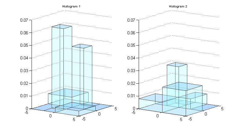
We can look at the subpaving or parition of the data space for each histogram and the union of these two subpavings, which is also a regular subpaving.
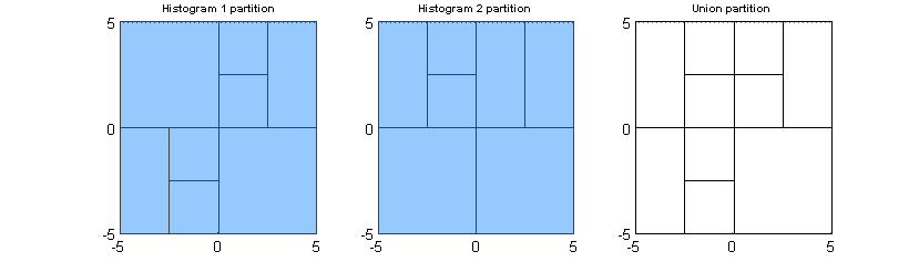
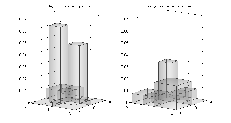
For each original histogram, a histogram of exactly the same shape but formed over the union subpaving can be found. Some of the bins have been subdivided but the height over the subdivided bin is the same as the height over the original larger bin and so the shape is the same (and the area of the histogram still integrates to 1). The images below show the result of representing the histograms to get the same shape but over the union subpaving.
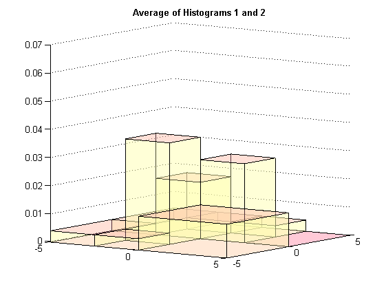
The average histogram is found by averaging the heights of the two histograms for each bin that is part of the union partion.
For examples using averaging and :AdaptiveHistogramCollator objects, see Example of averaging histograms and Example using data from a RSSample object.
In this example we show how an AdaptiveHistogram object can be used to process sample data from a Bivariate Gaussian distribution, ie two-dimensional data.
Our implementation of this example is in the file BiGTest.cpp, which includes the header file dataprep.hpp.
Dataprep.hpp specifies libaries for generating simulated random samples from statistical distributions
#ifndef ___DATAPREP_HPP__
#define ___DATAPREP_HPP__

#include <gsl/gsl_statistics_double.h>
#include <gsl/gsl_math.h>
#include <gsl/gsl_sort.h>
#include <gsl/gsl_statistics.h>
#include <gsl/gsl_rng.h>
#include <gsl/gsl_randist.h>

#endif
In BiGTest.cpp we include the other header files and libraries we want to be able to use. The file header histall.hpp includes the headers usually needed for programming using AdaptiveHistograms. We also specify the namespaces we want to be able to use without qualification.
#include <time.h>   // clock and time classes
#include <fstream>  // input and output streams

#include "histall.hpp"  // headers for the histograms
#include "dataprep.hpp" // headers for getting data

using namespace cxsc;
using namespace std;
using namespace subpavings;


int main()
{
The first part of the file is concerned with setting the up the objects to generate simulated random samples from a bivariate gaussian distribution.
    // ------- prepare to generate some data for the tests -----------

    // set up a random number generator for bivariate gaussian rvs
    const gsl_rng_type * T;
    gsl_rng * r;

    int i;
    const int n=10000;  // number to generate
    double sigma_x=1;   // distribution parameter
    double sigma_y=1;   // distribution parameter
    double rho=0;       // x and y uncorrelated

    //create a generator chosen by the environment variable GSL_RNG_TYPE

    gsl_rng_env_setup();

    T = gsl_rng_default;
    r = gsl_rng_alloc (T);
In this example, we put the samples generated into a txt file which will then be used to input data into the histogram. Note that when we create an ofstream object for the file to send the samples to, we specify the formatting for this to be scientific with precision. This ensures that each value output will include a decimal point.
    string samplesFileName; // for samples
    string outputFileName;// for output file
    ofstream oss;         // ofstream object
    oss << scientific;  // set formatting for input to oss
    oss.precision(5);

    double *x;
    double *y;

    x= new double[n];   // make x and y in dynamic memory
    y= new double[n];   // (so they must be freed later)

    double* itx;
    double* ity;


    // get n random variates chosen from the bivariate Gaussian
    // distribution with mean zero and given sigma_x, sigma_y.
    for (i = 0; i < n; i++)
    {
        gsl_ran_bivariate_gaussian(r, sigma_x, sigma_y,
                                   rho, &x[i], &y[i]);

    }

    // free the random number generator
    gsl_rng_free (r);
These are then output into a txt file. Note the format used in the section where we output the data to a txt file: Each pair of numbers is on the same line, separated by whitespace (in this case, just space, but tabs would also work).
    itx = &x[0];
    ity = &y[0];

    // create a name for the file to use
    samplesFileName = "bgSamples.txt";
    // output the sample data
    oss.open(samplesFileName.c_str());         // opens the file

    for(i=0; i<n; i++) {
        oss << (*itx) << "  " << (*ity);
        if (i<n-1) oss << endl; // new line if not final line
        itx++;
        ity++;
    }
    oss << flush;
    oss.close();

    cout << "Samples output to " << samplesFileName << endl << endl;
We also set up a way to time the processes, and some boolean variables used later in the process
    clock_t start, end;     // for timing
    double timeTaken;

    bool successfulInsertion = false;
    bool successfulPQSplit = false;
The first example in this file will show how to create a histogram with a rule to adjust the partition (split a node in the tree representing the subpaving partition) when the number of data points associated with the bin is greater than some number k. This is a simple implementation of an upper-bounded version of the statistically equivalent blocks (SEB) principle or test or rule.
    // ------ example to create one histogram with splitting value ----
    // --------------------entered by user ----------------------------
Pretending that we did not know how many data points were in the sample, we can find this out using the countLinesInTxt method and get an appropriate input value for k.
    // get a count of the lines in the txt file
    int dataCount = countLinesInTxt(samplesFileName);
    int myK = 0;

    // tell user how many lines there are in the file
    cout << "The file " << samplesFileName << " has " << dataCount
            << " lines in it" << endl << endl;
    // get a parameter for k
    cout << "Enter a parameter for your splitting criteria here please:  ";
    cin >> myK;
    cout << endl << endl; // myK has been input
Now we make the AdaptiveHistogram object, in this case rather unimaginatively called myHistFirst.
    // make an Adaptive Histogram object with no specified box and, by default,
    // holdAllStats = false so that the underlying rootPaving managed by the
    // histogram will not maintain all available stats, only counts
    AdaptiveHistogram myHistFirst;
myHist is given no initial values. This means that we have not actually specified a root box for the subpaving represented by the tree of SPSnodes that myHistFirst manages. This will be dealt with later by myHistFirst which will create a box tailor-made to fit all the data.
By default, the histogram data member holdAllStats is false.
Then we start a clock, to time how long processing the data takes.
    start=clock();
    // clock running
Now we create the function object to direct whether or not a node is split after a data point is associated with it.
    // make the function object to decide whether to split.
    // aim to get max myK data members in each box, default minimum
    // number of points allowed in each box is 0.
    SplitOnK splitK(myK);
See the class documentation for SplitOnK for more information on this object. Note that the minimum number of points to be associated with a node defaults to 0 in this example. If a minimum number of points to be associated with a node is specified in the SplitOnK constructor this would effectively override the specfified maximum k where there was a conflict between the two requirements. All nodes would have a least the minimum number of points but might have more than k data points associated with them because splitting the node would violate the minimum.
Next we input the data from the txt file of samples to myHistFirst, using the insertRvectorsFromTxtOrd method and supplying the function object splitK we have just created. We also specify that there will be no logging of the insertion process (see the enumeration LOGGING_LEVEL for possible values for the logging parameter).
    // insert the data on by one, checking whether to split on each insertion
    successfulInsertion = myHistFirst.insertRvectorsFromTxtOrd(samplesFileName,
            splitK, dim, headerlines, NOLOG); // no logging
This method returns a boolean (true or false) value indicating whether or not some data has been successfully read in, put in the the data collection, and presented to the StatsSubPaving managed by the histogram. In this case, because we did not initialise myHistFirst with a root box for the StatsSubPaving, a root box specifically tailored to the data will have been created as part of the data insertion process and so we will not have any data left out in the cold.
We now stop the clock and print out the processing time.
    end=clock();

    timeTaken = static_cast<double>(end-start)/CLOCKS_PER_SEC;
    cout << "Computing time : " <<timeTaken<< " s." << endl;
If the data insertion process was successful, we can output the subpaving to a txt file. The name of the file to send the output to is given in the program.
    // only do more if some data was fed in
    if(successfulInsertion) {

        // create a name for the file to output
        outputFileName = "BivGaussianFirst.txt";
        // To realize a file output
        myHistFirst.outputToTxtTabs(outputFileName);
Then we end the if statement checking if data insertion was successful and have finished the first example.
    }

    // end of example for histogram with splitting value input by user
The next part of the program demonstrates the priority queue method of forming the histogram: all the data is initially associated with the root box of the subpaving and a priority queue is then used to refine the bins in the partition.
    successfulInsertion = false;
    successfulPQSplit = false;

    // example to create one histogram with pulse data and a priority
    // ---------- split to give a minimum number of bins -----------
Again we make an AdaptiveHistogram object with no root box.
    // make an Adaptive Histogram object with no specified box
    // or splitting value (and holdAllStats again defaults to false),
    // with the same data
    AdaptiveHistogram myHistSecond;
We start the clock and insert the data, but this time we do not give any rule for splitting the subpaving as the data is inserted. The AdaptiveHistogram will simply make a root box big enough for all the data (because we have not pre-specified the root box) and will associate all the data with that box.
    start=clock();
    // clock running

    // put in the data in a 'pulse' with no splitting, ie one big box
    successfulInsertion = myHistSecond.insertRvectorsFromTxt(samplesFileName);
Now, provided that insertion of the data was successful, we do the actual formation of the histogram by the splitting the boxes most in need of attention first (ie, a priority queue).
In this example we specify that nodes should be compared on the basis of the number of data points associated with them by using a node comparision function object of type CompCount. This means that the node most in need of attention in the priority queue is the one with the largest number of data points associated with it.
We specifiy a stopping rule with a histogram evaluation function object of type CritLeaves_GTE. This object will stop the priority queue when the number of leaves in the tree representing the subpaving managed by the histogram is greater than or equal to 50.
The example also specifies a minimum number of data points that can be associated with any node in the tree. This requirement will effectively remove from the priority queue all nodes whose children would have less than 1 data point associated with them if the node were split. See Priority queue-based partitions and the AdaptiveHistogram::prioritySplit() method documentation for more information about the operation of this parameter.
    if (successfulInsertion) {

        // set up function objects for a priority split

        // function object to compare nodes on count
        // ie split node with largest count first
        CompCount compCount;

        // function object to split until number of leaves is >= minLeaves
        size_t minLeaves = 50;
        CritLeaves_GTE critLeavesGTE(minLeaves);

        /* minimum points to use when splitting.
        A node will not be splittable if either child would then have
        < minPoints of data associated with it. */
        size_t minPoints = 1;

        // do the priority split
        successfulPQSplit = myHistSecond.prioritySplit(compCount,
                critLeavesGTE, NOLOG, minPoints); // no logging
    }

    end=clock();
Then we show the time taken and output the histogram.
    timeTaken = static_cast<double>(end-start)/CLOCKS_PER_SEC;
    cout << "Computing time : " <<timeTaken<< " s." << endl;


    if(successfulPQSplit) { // only do more if split was successful

        // create a name for the file to output
        outputFileName = "BivGaussianSecond.txt";
        // To realize a file output
        myHistSecond.outputToTxtTabs(outputFileName);

    }
Free the memory allocated for the data points
    delete x;   // free dynamic memory used for x and y
    delete y;
And end the program
    return 0;

} // end of bivariate gaussian test program
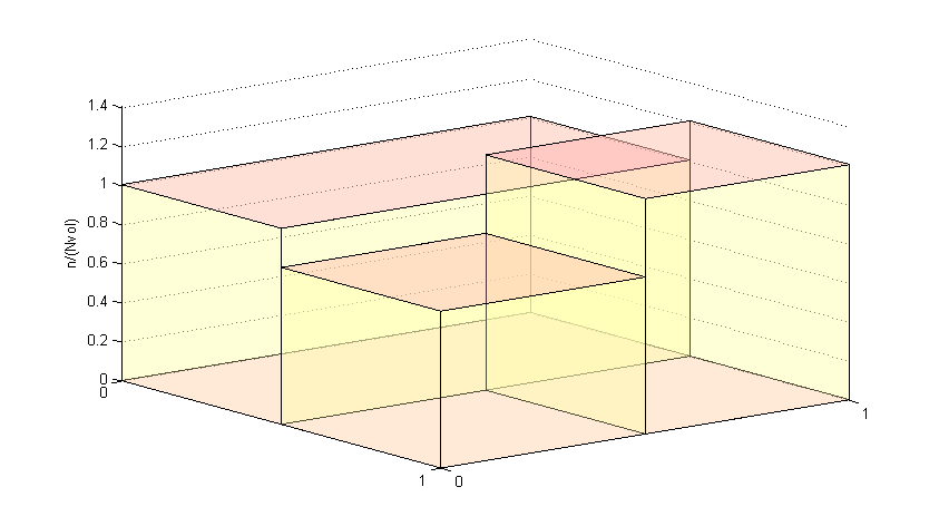
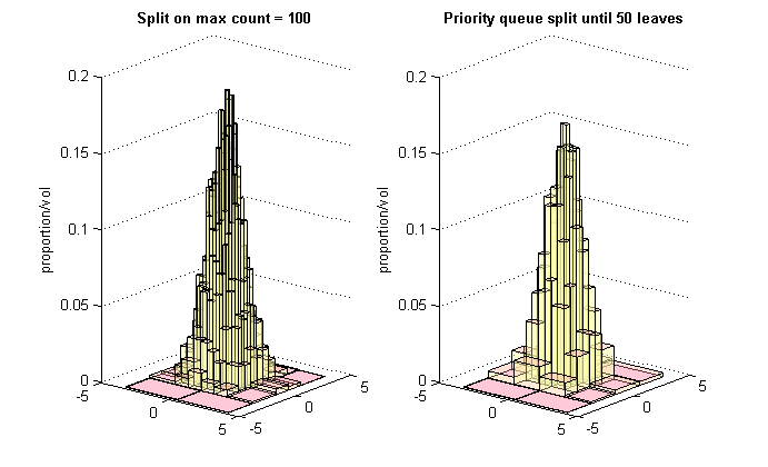
One of many possible displays of the result is shown below. This draws the histograms as 3-dimensional shapes, with the 'floor' being the boxes of the subpaving and the height of each histogram bar being the proportion of the total number of datapoints which were associated with that box divided by the floor area (volume of the box). The image shows both histograms, illustrating the smoothing effect achieved by priority queue splitting to a fixed number of leaves (bins in the partition).
In this example we show how an AdaptiveHistogramCollator object can be used find the average histogram from ten different histograms (AdaptiveHistogram objects), each managing a sample of bivariate gaussian data.
Our implementation of this example is in the file Averaging.cpp, which includes the header file dataprep.hpp.
Dataprep.hpp specifies libaries for generating simulated random samples from statistical distributions
In Averaging.cpp we also include the other header files and libraries we want to be able to use. The file header histall.hpp includes the headers usually needed for programming using AdaptiveHistograms. We also specify the namespaces we want to be able to use without qualification.
#include <time.h>   // clock and time classes
#include <fstream>  // input and output streams
#include <sstream>  // to be able to manipulate strings as streams

#include "histall.hpp"  // headers for the histograms
#include "dataprep.hpp" // headers for getting data

using namespace cxsc;
using namespace std;
using namespace subpavings;

int main()
{
The first part of the file is concerned with setting the file up to generate and store simulated random samples from a bivariate gaussian distribution.
    // ------- prepare to generate some data for the tests -----------

    // set up a random number generator for bivariate gaussian rvs
    const gsl_rng_type * T;
    gsl_rng * r;

    int i;
    const int n=10000;  // number to generate
    double sigma_x=1;   // distribution parameter
    double sigma_y=1;   // distribution parameter
    double rho=0;       // x and y uncorrelated

    //create a generator chosen by the environment variable GSL_RNG_TYPE

    gsl_rng_env_setup();

    T = gsl_rng_default;
    r = gsl_rng_alloc (T);
The example is described
    // ----------------   example to create and ------------------
    //---------------- collate multiple histograms -------------------
It is vital that each AdaptiveHistogram to be collated has the same root box, so we make a large root box which will be used by all the histograms we subsequently make.
    // make a box: the same box will be used by all histograms
    // so should be big enough for all of them
    int d = 2; // dimensions
    ivector pavingBox(d);
    interval dim1(-5,5);
    interval dim2(-5,5);
    pavingBox[1] = dim1;
    pavingBox[2] = dim2;
Then we make the AdaptiveHistogramCollator object
    // make a collation object, empty at present
    AdaptiveHistogramCollator coll;
We have a loop for each histogram to be averaged, and within the loop we start by generating sample data for the histogram. Note that the sample data is stored in a RVecData container.
    // the number of histograms to generate
    int numHist = 10;

    // for loop to generate histograms and add to collation
    for (int j=1; j<=numHist; j++) {

        //get n random variates chosen from the bivariate Gaussian
        // distribution with mean zero and given sigma_x, sigma_y.

        RVecData theData;   // a container for all the points generated

        // make a sample
        for (int i = 0; i < n; i++) {

            rvector thisrv(d);
            double x = 0;
            double y = 0;

            gsl_ran_bivariate_gaussian(r, sigma_x, sigma_y,
                                    rho, &x, &y);
            thisrv[1] = x;
            thisrv[2] = y;

            // put points generated into container
            theData.push_back(thisrv);

        }  // data should be in theData
We make an AdaptiveHistogram object to be used with this sample. Each histogram will use the a copy of the same root box for its subpaving.
        // make an Adaptive Histogram object with a specified box.  By default,
        // holdAllStats = false so that the underlying rootPaving managed by the
        // myHistFirst will not maintain all available stats, only counts
        AdaptiveHistogram myHist(pavingBox);
Each AdaptiveHistogram is to be formed under the rule where each bin should have a maximum number of data points k associated with it, but that maximum number of data points is a function of the total number of data points n and the histogram indexer j. This applies SEB heuristics for k to satisfy  as
as  . The resulting value for k is used in the constructor for an object of type SplitOnK. See the class documentation for SplitOnK for more information on this object. Note that the minimum number of points to be associated with a node defaults to 0.
        // find k, the maximum number of data members
        // to be allowed in each box of the histogram
        // as a function of j and n
        // applying SEB heuristics for k to satisfy k/n -> 0 as n -> +oo
        int k_int = (int(log2(double(n)))*2*j);

        cout << "Splitting with k = " << k_int << endl;

        bool successfulInsertion = false;
        bool successfulPQSplit = false;

        // make the function object to get max myK data members in each box
        SplitOnK splitK(k_int);
Next we input the sample data from the container into the histogram, using the insertFromRVec method and supplying the function object splitK we have just created. We also specify that there will be no logging of the insertion process (see the enumeration LOGGING_LEVEL for possible values for the logging parameter).
Note that we choose to split with each data insertion here. A priority queue with a stopping rule based on the maximum number of points associated with any any leaf node of the tree (CritLargestCount_LTE) could also be used.
        // insert data into the histogram, splitting as we go, no logging
        successfulInsertion = myHist.insertFromRVec(theData, splitK, NOLOG);
Assuming that the data insertion has been successful, we output each histogram to a txt file and add it to the collation.
Adding the histogram to the collation does not change the AdaptiveHistogram object itself, it just adds information from that object to the collation.
A dot file of the tree representation of the histogram can also be created but works best for smaller histograms.
        // only do more if some data was fed in
        if(successfulInsertion) {

            // create a name for the file to output
            string fileName = "BivGaussian";
            //convert j to a string
            std::ostringstream stm2;
            stm2 << j;
            // add the stringed j to the filename
            fileName += stm2.str();
            fileName += ".txt"; // and finish the filename

            // To realize a file output
            myHist.outputToTxtTabs(fileName);

            // add the histogram to the collection
            coll.addToCollation(myHist);

            // optional- create graph output
            // myHist.outputGraphDot();
        }
This ends the loop for creating separate histogram objects. The random number generator can be freed.
    } // end of for loop creating histograms

    // free the random number generator
    gsl_rng_free (r);
And the collated information output to a txt file. A dot graph can also be created if desired.
    string collfileName = "CollatorHistogram.txt";
    coll.outputToTxtTabs(collfileName); // output the collation to file

    // optional - create graph output - don't do for lots of leaves!
    //coll.outputGraphDot();
Finally, the average is also output to a txt file.
  //  Make an average
  string avgfileName = "AverageBG.txt";     // provide a filename

  AdaptiveHistogramCollator avColl = coll.makeAverage();
  avColl.outputToTxtTabs(avgfileName);  // output the average to file
The example ends.
    // ---- end of example to create and collate multiple histograms -----

    return 0;

} // end of averaging test program
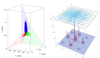
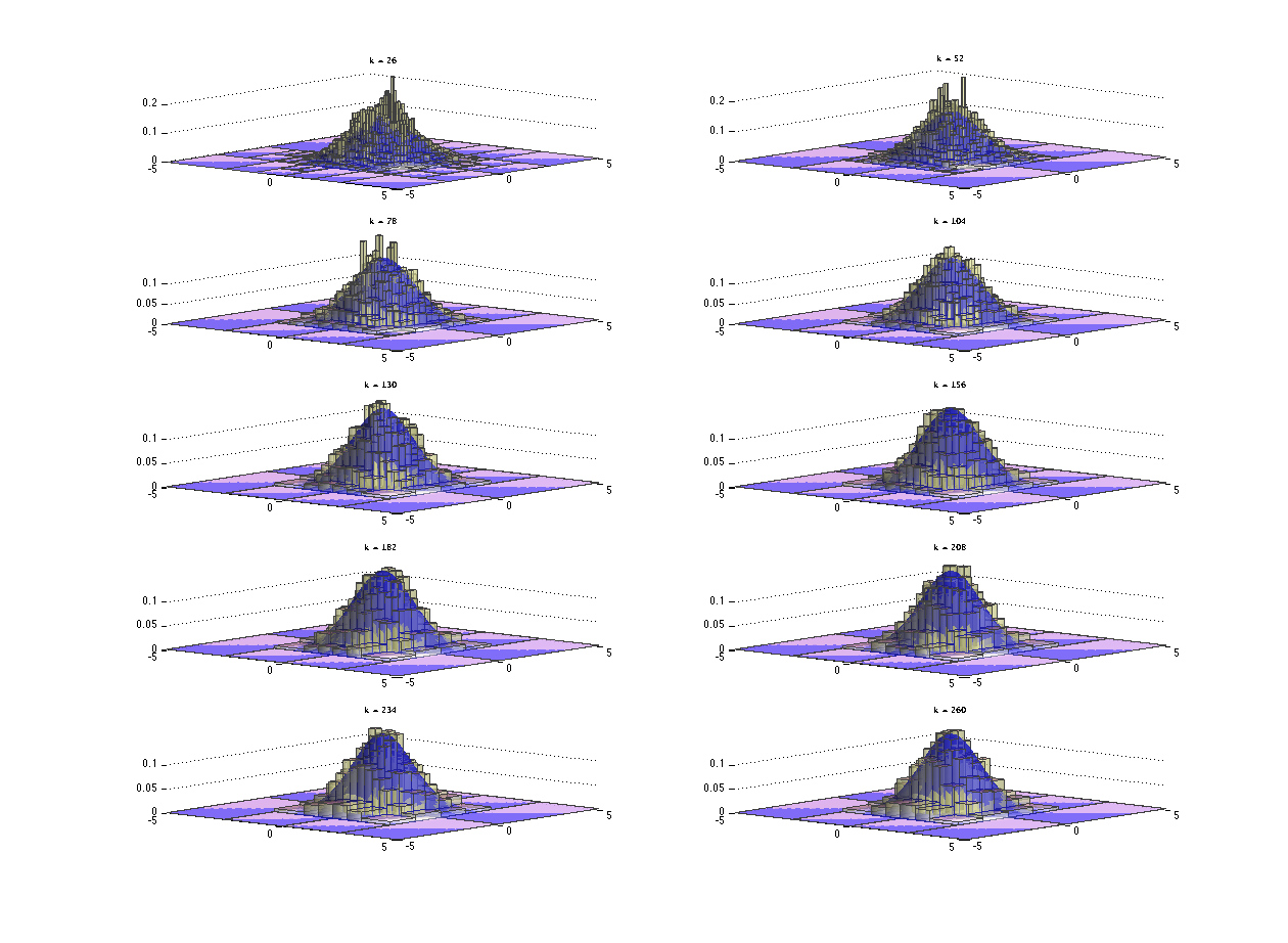
The ten histograms constructed with different values of k based on the ten independent simulations of 10000 bivariate Gaussian samples are diplayed next along with the prabability density of the standard bivariate Gaussian.
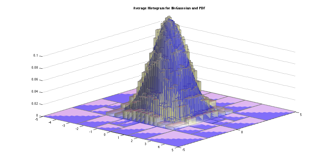
The average histogram or the sample mean histogram of the above 10 histograms are shown below with the probability density of the standard bivariate Gaussian.
This example first generates data in an RSSample object and then inputs samples from this to an AdaptiveHistogram, again averaging the resulting histograms.
The example must include the header files for the rejection sampling process
#include <time.h>   // clock and time classes
#include <fstream>  // input and output streams
#include <sstream>  // to be able to manipulate strings as streams

#include "histall.hpp"  // headers for the histograms

#include <gsl/gsl_qrng.h>       // types needed by MRSampler.hpp
#include <gsl/gsl_randist.h>
#include "Fobj.hpp"     // to be able to use the Levy function objects
#include "FLevy2D.hpp"
#include "MRSampler.hpp"    // to be able to do MRS rejection sampling


using namespace cxsc;
using namespace std;
using namespace subpavings;

bool collateFromRSSampleSplitPQ(AdaptiveHistogramCollator& coll,
          size_t samplesize, size_t numberSamples,
          const RSSample rss,
                    ivector pavingBox, const NodeCompObj& compTest,
                    const HistEvalObj& he,
                    size_t minChildPoints, double minVolB, int label);

int main (int argc, char **argv)
{

    // example to average 10 samples from a 2-d Levy shape
We start by using the Moore Rejection Sampler to generate the RSSample of data. See Moore Rejection Sampler for more information.
    ios::sync_with_stdio (); // so iostream works with stdio
    cout << SetPrecision (20, 15);  // Number of mantissa digits in I/O


    int n_dimensions = 2;
    int n_boxes = 1000;
    int n_samples = 100000;
    double Alb = 1.0;// partition until lower bound on Acceptance Prob.>Alb
    unsigned theSeed = 12345;


    bool use_f_scale = true;

    cout << "# n_dimensions: " << n_dimensions << "  n_boxes: " << n_boxes
        << "  n_samples: " << n_samples << "  rng_seed = " << theSeed
        << endl; //getchar();

    //Parameters specific to the Levy target
    real Temperature = 40.0;
    real Center1 = 1.42513;
    real Center2 = 0.80032;
    real GlobalMax = 176.14;
    real DomainLimit = 10.0;    //0.999999999999999;
    bool UseLogPi = false; // log scale won't work naively

    // make the function object
    FLevy2D F_Levy_Temp_2D(Temperature, GlobalMax,
                        Center1, Center2, DomainLimit, UseLogPi);

    // create the sampler
    MRSampler theSampler (F_Levy_Temp_2D, n_boxes, Alb, theSeed,
                        (use_f_scale == 1));

    // produce the samples (n_sample samples should be produced)
    RSSample rs_sample; // object for the sample

    theSampler.RejectionSampleMany (n_samples, rs_sample);
We make a root box which will be used by all the histograms to be averaged.
    // make a box: the same box will be used by all histograms
    // so should be big enough for all of them, so use the function domain
    // set up the domain list
    ivector pavingBox(2);
    interval dim1(-DomainLimit, DomainLimit);
    interval dim2(-DomainLimit, DomainLimit);
    pavingBox[1] = dim1;
    pavingBox[2] = dim2;
We specify how many data points are to go into each sample and how many histograms to average over, then make an AdaptiveHistogramCollator to collate the separate histograms together.
    size_t samplesize = 10000; // number of samples to take from the RSSample

    // the number of histograms to generate
    size_t numSamples = 10;

    // make a collation object, empty at present
    AdaptiveHistogramCollator coll;
We will use a single method of the AdaptiveHistogramCollator object to both create each histogram using priority queue splitting and collate the histograms.
For this we need to set up function objects and other arguments to be used in the priority queue operations.
In this example we specify that nodes should be compared on the basis of the number of data points associated with them by using a node comparision function object of type CompCount. This means that the node most in need of attention in the priority queue is the one with the largest number of data points associated with it.
We specifiy a stopping rule with a histogram evaluation function object of type CritSmallestVol_LTE. This object is constructed to stop a priority queue when the volume of the smallest box in the subpaving (partition) is less than 0.05.
We could specify a minimum number of data points that can be associated with any node in a tree. In this example we set this to 0 which will have no effect on the priority queue operations. Similarly we use minVolB = 0.0 to specify no minimum volume for the boxes represented by nodes in the trees. See Priority queue-based partitions and the AdaptiveHistogram::prioritySplit() method documentation for more information about the operation of these arguements.
    // set up objects for priority queue splitting

    // node comparison using count of data points associated with nodes
    CompCount compCount;

    // stopping on smallest volume criteria for splittable nodes
    double vol = 0.05;
    CritSmallestVol_LTE critSmallestVol(vol);

    /* A node is not splittable if splitting that node would give at least
    one child with < minPoints of data associated with it.*/
    size_t minPoints = 0;

    /* minVolB is the multiplier for (log n)^2/n to determine the minumum
    volume for a splittable node where n is total points in subpaving.
    A node with volume < minVolB(log n)^2/n will not be splittable. */
    double minVolB = 0.0;
The actual creation of the 'sample' histograms and their collation into the AdaptiveHistogramCollator is carried out using the collateFromRSSampleSplitPQ method. If the method is successful, it will output a separate txt file for each 'sample' histogram. The collated results will be in the AdaptiveHistogramCollator we have named "coll" (this is output to the txt file CollatorHistogram.txt). The average is also created and output to AverageHistogram.txt.
    bool success = collateFromRSSampleSplitPQ(coll,
          samplesize, numSamples,
                    rs_sample, pavingBox, compCount,
                    critSmallestVol, minPoints, minVolB,
          label);

  if (success) {
            string fileName = "CollatorHistogram.txt";
            coll.outputToTxtTabs(fileName); // output the collation to file

            //  Average the histograms
            fileName = "AverageHistogram.txt";     // provide a filename

            coll.outputAverageToTxtTabs(fileName);  // output the average to file
    }

    else    cout << "Failed to create collation over histograms" << endl;
The example program then ends.
    return 0;

} // end of Levy test program
This is an example of a section of code which sets up an AdaptiveHistogram object by specifying the root box (the interval [-40.0 40.0]) as well as the splitting value (2) and then defines the data within the program code and feeds each value individually to the AdaptiveHistogram. It is unlikely that this method would be useful in most practical circumstances but the example is included to illustrate the use of the pre-specified root box and the insertOne() method.
  ivector x(1);
  x[1] = interval(-40.0, 40.0);

  AdaptiveHistogram myHist(x);

  size_t k = 2;
  // function object to split when > 2 data points associated with a node
  SplitOnK splitDecision(k);

  real newreal = -3.0;
  // one dimensional rvector, only element is newreal
  myHist.insertOne(newdata, splitDecision);

  newreal = 14.0;
  newdata = _rvector(newreal); // another one
  myHist.insertOne(newdata, splitDecision);

  newreal = 6.0;
  newdata = _rvector(newreal); // another one
  myHist.insertOne(newdata, splitDecision);

  newreal = -10.0;
  newdata = _rvector(newreal); // another one
  myHist.insertOne(newdata, splitDecision);

  newreal = -3.0;
  newdata = _rvector(newreal); // another one
  myHist.insertOne(newdata);
The AdaptiveHistogram class has not yet been fully developed. More methods and functionality can be usefully added.
More flexible user friendly input and output
Generate graphical output for histograms